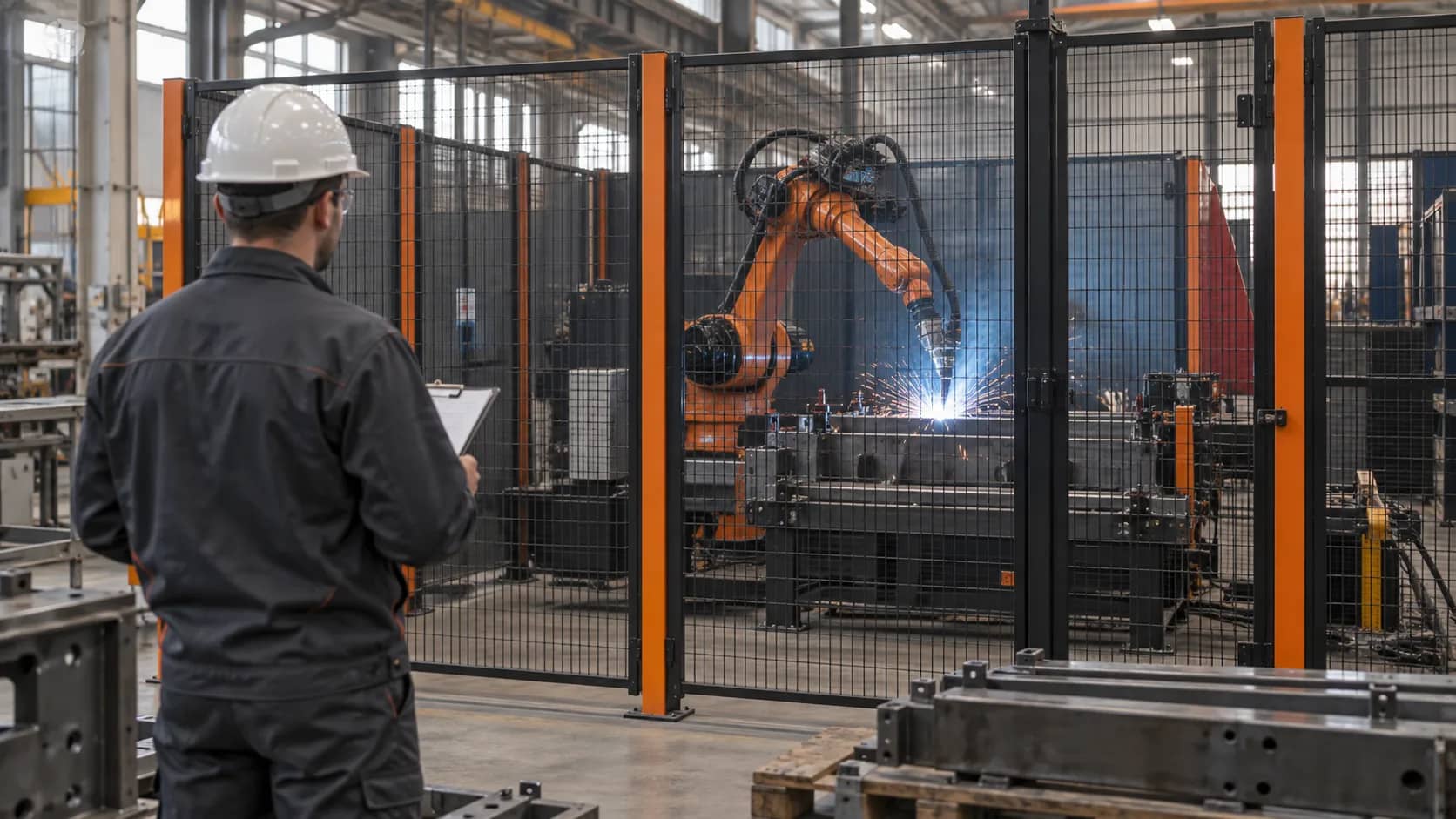
Measure the present process before modeling ROI
Start with twelve months of actual good-part output, paid welding and handling hours, scrap/rework, stoppages and changeovers. Note customer demand and the downstream constraint. If a robot shortens weld time but inspection or material supply remains the bottleneck, the resulting theoretical capacity is not automatically saleable output.
Record the proposed cell's full boundary: robot, weld package, fixture, safety, site preparation, integration, FAT/SAT, freight, training and startup. The companion welding-cell cost guide provides an inclusion/exclusion matrix so this model does not omit capital paid by the plant rather than the supplier.
- Baseline good units and demanded additional units by part family
- Measured full cycle, availability, planned maintenance and changeover
- Loaded paid labor hours that can actually be removed or redeployed to a valued task
- Avoidable rework cost after inspection and scrap accounting
- One-time project spend and recurring operating expense
Three ways an ROI claim can overstate value
Use good units with confirmed demand and downstream room, not theoretical robot cycles.
Subtract variable cost; use contribution per additional saleable unit.
A worker moved to another task is not a payroll saving unless its value is separately demonstrated.
A reproducible robotic welding ROI equation
Annual gross benefit = (additional saleable good units × contribution per unit) + (released paid hours × loaded hourly cost) + avoidable rework/scrap spend. Annual net benefit = gross benefit − incremental recurring cost. Simple payback after ramp-up is the time for cumulative net benefit to recover full one-time investment; if annual net benefit is zero or negative, this simple model has no payback.
Never count the same benefit twice. If labor is reassigned to make the extra units, do not also claim a cash wage reduction for those hours. If rework reduction is already reflected in additional good units, include only the remaining separately avoidable cost. Contribution margin excludes variable production costs; revenue is not margin.
- Show units and currency beside every input; keep source and owner of each assumption.
- Use a first-year ramp factor for commissioning, training and part-family release, while retaining fixed annual costs.
- For irregular cash flow, use a year-by-year cumulative schedule; do not substitute a single steady-state ratio.
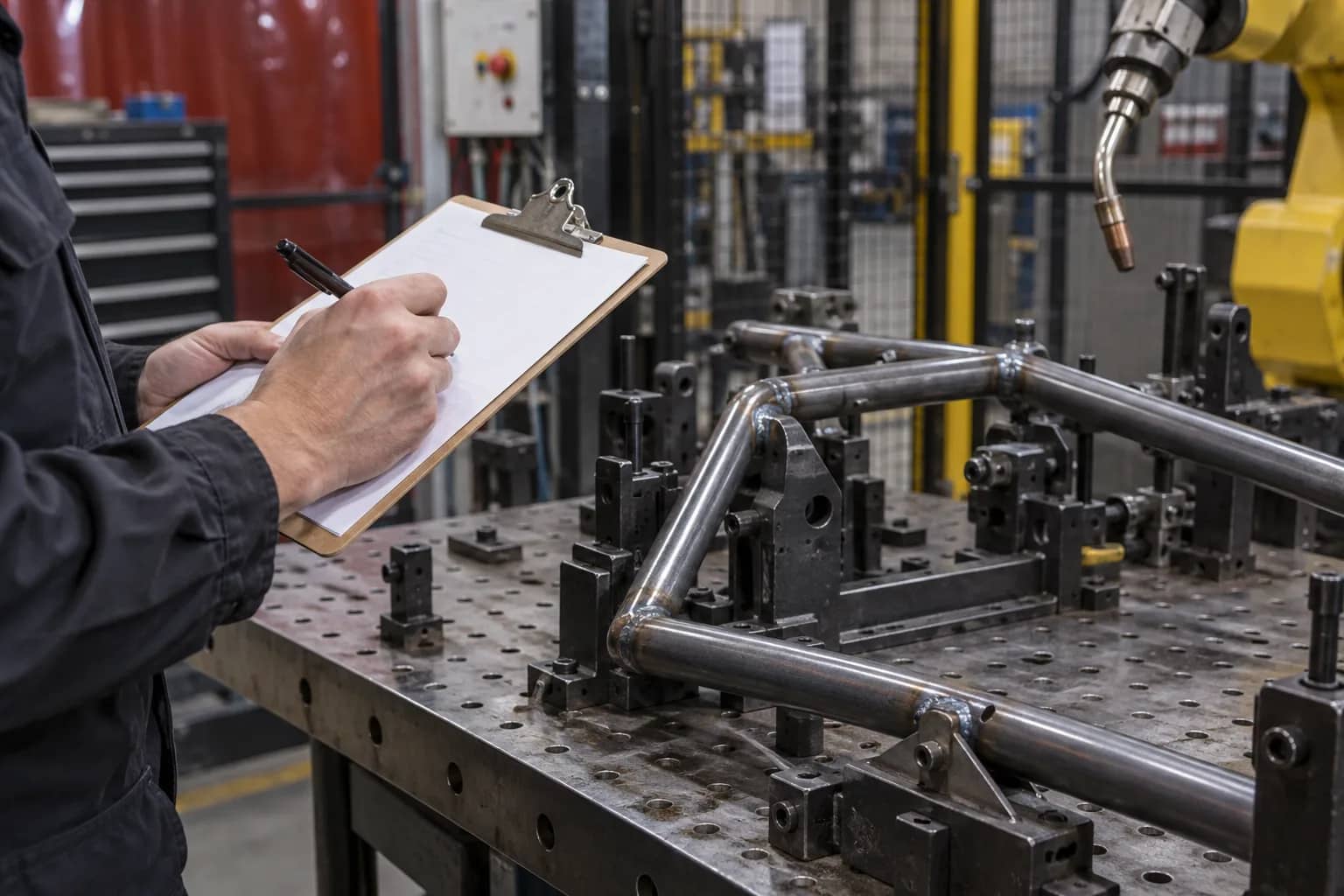
Worked example — assumptions, not a forecast
Suppose a proposed cell and all required site work cost USD 240,000. Assume 6,000 additional good units per stabilized year with USD 18 contribution per unit, 800 paid hours genuinely released at USD 28/hour, and USD 12,000 of separately measured avoidable rework. Annual added maintenance, power, consumables and programming total USD 32,000. These are invented teaching inputs; they do not describe TubeFrame's prices, capacity or results.
Gross annual benefit is 6,000 × 18 + 800 × 28 + 12,000 = USD 142,400. Stabilized annual net benefit is USD 110,400. If first-year benefits achieve only 60% of the stabilized level while the full USD 32,000 operating cost is incurred, first-year net benefit is USD 53,440. Remaining investment after year one is USD 186,560; at the assumed stabilized rate, illustrative simple payback is about 2.69 years. Do not use that answer for a purchasing decision without actual plant inputs.
- Demand and downstream capacity must support all 6,000 extra good units.
- The 800 hours must be a real cash saving or separately valued redeployment—not both.
- No discount rate, tax, financing, price change or residual value is modeled.
Evidence flow for the investment case
Current good units and cost
Cell + full project cost
Cycle, quality and uptime
Cash benefits − recurring costs
Downside and acceptance gates
Test the downside before trusting payback
Now halve the additional good units to 3,000, halve released paid hours to 400 and rework savings to USD 6,000, while annual running cost rises to USD 40,000. The same USD 240,000 upfront spend then produces only USD 31,200 stabilized annual net benefit. With the same 60% first-year benefit ramp, first-year net is USD 2,720 and illustrative payback extends to about 8.61 years.
The swing is not a prediction. It shows why good-unit demand, weld access, fit-up, station loading, changeover and uptime should be validated with actual parts and pilot evidence. A3's general robot calculator and welding-specific guidance from BP Automation and Tregaskiss identify many of these inputs; this worksheet makes the dependencies visible to a buyer.
- Vary demand, contribution, labor realization, rework and operating costs separately.
- Treat safety improvements and ergonomics as decision factors, but do not invent a cash value.
- If capital approval requires discounted cash flow, use the company's approved rate and finance method.
What to send for an evidence-led proposal
Send representative drawings or samples, current shift records, weld and inspection criteria, part-family mix, target good output, layout and utility constraints. Ask the supplier which performance assumptions require a trial, simulation, FAT or SAT result. Request the proposed scope and acceptance plan before updating your investment model.
See the robotic welding application for configuration choices, the welding-cell cost guide for quote boundaries and the request-a-quote page to begin a review. TubeFrame can coordinate a project-specific configuration and delivery discussion; it cannot guarantee this example's output or payback.
Example input sheet and sensitivity
Every value in this table is an example assumption in USD, not a TubeFrame quotation, real project result or guaranteed outcome. Replace it with measured plant data.
Copy the rows into your RFQ or investment worksheet.
| Input | Base example | Downside example | Verification question |
|---|---|---|---|
| Full upfront investment | USD 240,000 | USD 240,000 | Does this include site work, training and acceptance? |
| Extra good units / year | 6,000 | 3,000 | Demanded and deliverable after downtime? |
| Contribution / good unit | USD 18 | USD 18 | Finance-approved after variable costs? |
| Released paid hours / year | 800 h | 400 h | Actual payroll reduction or valued redeployment? |
| Loaded hourly cost | USD 28/h | USD 28/h | Recorded plant rate? |
| Avoidable rework / year | USD 12,000 | USD 6,000 | Not already counted in good units? |
| Added annual operating cost | USD 32,000 | USD 40,000 | Maintenance, power, consumables, programming? |
| First-year benefit ramp | 60% | 60% | Commissioning and part release evidence? |
| Stabilized annual net | USD 110,400 | USD 31,200 | Recalculate from rows above. |
| Illustrative simple payback | ≈2.69 years | ≈8.61 years | Not a promised or discounted return. |
Frequently asked questions
What is the quickest valid payback check?
Compare full upfront spend with cumulative annual cash benefit after incremental recurring costs. Apply a ramp-up year and a downside case; if steady annual net is non-positive, this simple model does not pay back.
Should added output be valued at sales price?
No. Count only additional good units that can actually be sold and delivered. Multiply by contribution after variable costs, not by gross sales price.
Can I count both labor savings and extra production?
Only if they are separate realized benefits. Do not count the same operator hours as both payroll reduction and labor used to make additional output.
Does this example guarantee a 2.69-year payback?
No. Every number is an illustrative assumption. Actual results depend on demand, part consistency, cell performance, operating cost and the agreed delivery scope.
Original sources and model boundaries
Validate the inputs before committing capital
Send the workpiece, current good-output and quality records, target demand and site constraints. Request a cell scope and validation plan before replacing the example inputs.
Discuss a welding project ↗